In order to present results as realistic as possible in our PAA-paper, we constructed long-term end-of-month data series for popular ETF proxies, like SPY, GLD and TLT (see paper appendix on SSRN). All data series start December 1969. For the pre-inception history, the proxies are derived from suitable indices. As part of a complete revision of the long-term data set, we recently improved the construction of the data series by mapping the underlying index through a linear formula to arrive at the best fit over the life span of the ETF to be replicated. The construction process is demonstrated below for EFA. The link to an example spreadsheet with all the necessary calculations is published at the end of this post.
EFA seeks to track the investment results of the MSCI EAFE index which is composed of large- and mid-capitalization developed market equities, excluding the U.S. and Canada. The index data is available as free download from the MSCI website. Comparing EFA’s historical data record against the various index levels supported by MSCI like Price, Gross, Net, reveals the MSCI EAFE Net index as underlying index. Historical dividend adjusted data for EFA itself is offered by Yahoo Finance, also for free. For constructing a long-term EFA proxy the data from both sources is required.
With the data readily available in Excel, the next step is to derive the data for the ETF-proxy from the underlying index for the In-Sample (IS) period. The goal is to map the underlying to arrive at the best fit over the life span (=IS) of the ETF through a linear formula: r+ = b * r + a, where “r” is the return of the index and “r+” is the return for the proxy. The values for the coefficients “a” and “b” are determined through Excel’s Solver add-in by minimizing the unexplained sum of squared deviations for the return series of EFA and the ETF-proxy.
After Solver finishes the calculation cycles, the found coefficients result in high R-Squared and correlation readings.
Visual inspection of the resulting curves shows a high degree of fit with minimal distortions.
The found mapping formula can be checked by plotting the return series of MSCI EAFE and EFA as scatter graph with the linear regression line overlaid. The coefficients of the regression line match with the ones derived by Solver. Hence the scatter graph approach offers a handy shortcut, making the Solver approach essentially superfluous.
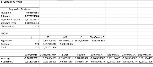
Furthermore the results may be double-checked by a regression analysis through Excel’s Analysis Toolpak add-in. The low Significance F reading (below 0.05) shows the found coefficients are reliable (statistically significant).
Having found statistically significant coefficients for the IS period (2001-2015), EFA's history can now be extended for the Out-of-Sample period, back to the inception date of the MSCI EAFE index: December 1969. The final result is a proxy for EFA covering 1969 - 2015: "EFA+"
After following the same workflow for other ETF’s, the final result is a collection of data series in Excel like the below sample (DummyData.xlsx):
To export the data from Excel and save each ETF-proxy in its separate csv-file, the following [updated] R-code comes in handy. The code adds a $-prefix to each ETF’s name for distinction.
[Update:] Hat tips to Adam Butler and Carlos Espeleta for pointing at the openxlsx package for R, which removes the Java dependent package previously used.
The output of the R-code is a collection of csv-files with dates and closes, ready for import in your charting program.
Sources of interest:
- Yahoo Finance
- MSCI
- NAREIT
- Fama/French
- Deutsche Bank IQ
- Quandl
- Morningstar
- Barchart
- Norgate Data
- Mike Middleton
The example spreadsheet along with the R-code and the DummyData.xlsx files are available on the Google Drive folder connected to this post.


